
Low Level Interface#
For more advanced use, it can be useful to have access to lower-level internals of the CoolProp code. For simpler use, you can use the high-level interface. The primary reason why this low-level interface is useful is because it is much faster, and actually the high-level interface internally calls the low-level interface. Furthermore, the low-level-interface exclusively operates using enumerated values (integers) and floating point numbers, and uses no strings. String comparison and parsing is computationally expensive and the low-level interface allows for a very efficient execution.
At the C++ level, the code is based on the use of an AbstractState abstract base class which defines a protocol that the property backends must implement. In this way, it is very easy to extend CoolProp to connect with another completely unrelated property library, as was done for REFPROP. As long as the interface to the library can be coerced to work within the AbstractState structure, CoolProp can interface seamlessly with the library.
In order to make most effective use of the low-level interface, you should instantiate one instance of the backend for each fluid (or mixture), and then call methods within the instance. There is a certain amount of computational overhead in calling the constructor for the backend instance, so in order to minimize it, only call the constructor once, and pass around your class instance.
Warning
While the warning about the computational overhead when generating AbstractState instances is more a recommendation, it is required that you allocate as few AbstractState instances as possible when using the tabular backends (TTSE & Bicubic).
Warning
In C++, the AbstractState::factory() function returns a bare pointer to an AbstractState instance, you must be very careful with this instance to make sure it is appropriately destroyed. It is HIGHLY recommended to wrap the generated instance in a shared pointer as shown in the example. The shared pointer will take care of automatically calling the destructor of the AbstractState when needed.
Similar methodology is used in the other wrappers of the low-level interface to (mostly) generate 1-to-1 wrappers of the low-level functions to the target language. Refer to the examples for each language to see how to call the low-level interface, generate an AbstractState instance, etc.
Introduction#
To begin with, an illustrative example of using the low-level interface in C++ is shown here:
#include "CoolProp.h"
#include "AbstractState.h"
#include <iostream>
#include "crossplatform_shared_ptr.h"
using namespace CoolProp;
int main() {
    shared_ptr<AbstractState> Water(AbstractState::factory("HEOS", "Water"));
    Water->update(PQ_INPUTS, 101325, 0);  // SI units
    std::cout << "T: " << Water->T() << " K" << std::endl;
    std::cout << "rho': " << Water->rhomass() << " kg/m^3" << std::endl;
    std::cout << "rho': " << Water->rhomolar() << " mol/m^3" << std::endl;
    std::cout << "h': " << Water->hmass() << " J/kg" << std::endl;
    std::cout << "h': " << Water->hmolar() << " J/mol" << std::endl;
    std::cout << "s': " << Water->smass() << " J/kg/K" << std::endl;
    std::cout << "s': " << Water->smolar() << " J/mol/K" << std::endl;
    return EXIT_SUCCESS;
}
which yields the output:
T: 373.124 K
rho': 958.367 kg/m^3
rho': 53197.5 mol/m^3
h': 419058 J/kg
h': 7549.44 J/mol
s': 1306.92 J/kg/K
s': 23.5445 J/mol/K
This example demonstrates the most common application of the low-level interface. This example could also be carried out using the high-level interface with a call like:
PropsSI("T", "P", 101325, "Q", 1, "Water")
Generating Input Pairs#
A listing of the input pairs for the AbstractState::update() function can be found in the source documentation at CoolProp::input_pairs. If you know the two input variables and their values, but not their order, you can use the function CoolProp::generate_update_pair() to generate the input pair.
Warning
The syntax for this function is slightly different in python since python can do multiple return arguments and C++ cannot.
A simple example of this would be
In [1]: import CoolProp

In [2]: CoolProp.CoolProp.generate_update_pair(CoolProp.iT, 300, CoolProp.iDmolar, 1e-6)
Out[2]: (11, 1e-06, 300.0)

In [3]: CoolProp.DmolarT_INPUTS
Out[3]: 11
Keyed output versus accessor functions#
The simple output functions like AbstractState::rhomolar() that are mapped to keys in CoolProp::parameters can be either obtained using the accessor function or by calling AbstractState::keyed_output(). The advantage of the keyed_output function is that you could in principle iterate over several keys, rather than having to hard-code calls to several accessor functions. For instance:
In [4]: import CoolProp

In [5]: HEOS = CoolProp.AbstractState("HEOS", "Water")

In [6]: HEOS.update(CoolProp.DmolarT_INPUTS, 1e-6, 300)

In [7]: HEOS.p()
Out[7]: 0.002494311404279685

In [8]: [HEOS.keyed_output(k) for k in [CoolProp.iP, CoolProp.iHmass, CoolProp.iHmolar]]
Out[8]: [0.002494311404279685, 2551431.0685640117, 45964.71448370705]
Things only in the low-level interface#
You might reasonably ask at this point why we would want to use the low-level interface as opposed to the “simple” high-level interface. In the first example, if you wanted to calculate all these output parameters using the high-level interface, it would require several calls to the pressure-quality flash routine, which is extremely slow as it requires a complex iteration to find the phases that are in equilibrium. Furthermore, there is a lot of functionality that is only accessible through the low-level interface. Here are a few examples of things that can be done in the low-level interface that cannot be done in the high-level interface:
In [9]: import CoolProp

In [10]: HEOS = CoolProp.AbstractState("HEOS", "Water")

# Do a flash call that is a very low density state point, definitely vapor
In [11]: %timeit HEOS.update(CoolProp.DmolarT_INPUTS, 1e-6, 300)
3.48 us +- 3.48 ns per loop (mean +- std. dev. of 7 runs, 100,000 loops each)

# Specify the phase - for some inputs (especially density-temperature), this will result in a
# more direct evaluation of the equation of state without checking the saturation boundary
In [12]: HEOS.specify_phase(CoolProp.iphase_gas)

# We try it again - a bit faster
In [13]: %timeit HEOS.update(CoolProp.DmolarT_INPUTS, 1e-6, 300)
3.46 us +- 8.19 ns per loop (mean +- std. dev. of 7 runs, 100,000 loops each)

# Reset the specification of phase
In [14]: HEOS.specify_phase(CoolProp.iphase_not_imposed)

# A mixture of methane and ethane
In [15]: HEOS = CoolProp.AbstractState("HEOS", "Methane&Ethane")

# Set the mole fractions of the mixture
In [16]: HEOS.set_mole_fractions([0.2,0.8])

# Do the dewpoint calculation
In [17]: HEOS.update(CoolProp.PQ_INPUTS, 101325, 1)

# Liquid phase molar density
In [18]: HEOS.saturated_liquid_keyed_output(CoolProp.iDmolar)
Out[18]: 18274.94908936083

# Vapor phase molar density
In [19]: HEOS.saturated_vapor_keyed_output(CoolProp.iDmolar)
Out[19]: 69.50308285938863

# Liquid phase mole fractions
In [20]: HEOS.mole_fractions_liquid()
Out[20]: [0.00610679002150561, 0.9938932099784945]

# Vapor phase mole fractions -
# Should be the bulk composition back since we are doing a dewpoint calculation
In [21]: HEOS.mole_fractions_vapor()
Out[21]: [0.2, 0.8]
Imposing the Phase (Optional)#
Each call to update() requires the phase to be determined based on the provided input pair, and may require a non-trivial flash calculation to determine if the state point is in the single-phase or two-phase region. For computational efficiency, CoolProp provide a facility to manually impose the phase before updating the state point. As demonstrated above, specifying the phase of a state point can result in a speed-up of ~10%, depending on the input pair provided and the phase region specified. If unspecified, CoolProp will determine the phase.
Depending on the input pair, there may or may not be a speed benefit to imposing a phase, like the one demonstrated above for DmolarT_INPUTS. If, for a given input pair, there is little or no speed benefit, or if the flash calculation has to be performed anyway to determine saturation values, the imposed phase may simply be ignored internally.
To specify the phase to be used, the AbstractState provides the following function:
# Imposing the single-phase gas region
In [22]: HEOS.specify_phase(CoolProp.iphase_gas)
The specified phase parameter can be one of the CoolProp constants in the table below.
Phase Constant |
Phase Region |
|---|---|
iphase_liquid |
p < pcrit & T < Tcrit ; above saturation |
iphase_gas |
p < pcrit & T < Tcrit ; below saturation |
iphase_twophase |
p < pcrit & T < Tcrit ; mixed liquid/gas |
iphase_supercritical_liquid |
p > pcrit & T < Tcrit |
iphase_supercritical_gas |
p < pcrit & T > Tcrit |
iphase_supercritical |
p > pcrit & T > Tcrit |
iphase_not_imposed |
(Default) CoolProp to determine phase |
To remove an imposed phase and allow CoolProp to determine the phase again, one of the following calls can be made.
# Reset the specification of phase
In [23]: HEOS.specify_phase(CoolProp.iphase_not_imposed)

# Or, more simply
In [24]: HEOS.unspecify_phase()
Phase specification in the low-level interface should be performed right before the call to update().
Warning
When specifying an imposed phase, it is absolutely critical that the input pair actually lie within the imposed phase region. If an incorrect phase is imposed for the given input pair, update() may throw unexpected errors or incorrect results may possibly be returned from the property functions. If the state point phase is not absolutely known, it is best to let CoolProp determine the phase at the cost of some computational efficiency.
Partial Derivatives#
It is possible to get the partial derivatives in a very computationally efficient manner using the low-level interface, using something like (python here):
For more information, see the docs: CoolProp::AbstractState::first_partial_deriv() and CoolProp::AbstractState::second_partial_deriv()
In [25]: import CoolProp

In [26]: HEOS = CoolProp.AbstractState("HEOS", "Water")

In [27]: HEOS.update(CoolProp.PT_INPUTS, 101325, 300)

In [28]: HEOS.cpmass()
Out[28]: 4180.6357765560715

In [29]: HEOS.first_partial_deriv(CoolProp.iHmass, CoolProp.iT, CoolProp.iP)
Out[29]: 4180.6357765560715

In [30]: %timeit HEOS.first_partial_deriv(CoolProp.iHmass, CoolProp.iT, CoolProp.iP)
142 ns +- 1.45 ns per loop (mean +- std. dev. of 7 runs, 10,000,000 loops each)

# See how much faster this is?
In [31]: %timeit CoolProp.CoolProp.PropsSI('d(Hmass)/d(T)|P', 'P', 101325, 'T', 300, 'Water')
844 us +- 830 ns per loop (mean +- std. dev. of 7 runs, 1,000 loops each)

In [32]: HEOS.first_partial_deriv(CoolProp.iSmass, CoolProp.iT, CoolProp.iDmass)
Out[32]: 13.767247481715131

# In the same way you can do second partial derivatives
# This is the second mixed partial derivative of entropy with respect to density and temperature
In [33]: HEOS.second_partial_deriv(CoolProp.iSmass, CoolProp.iT, CoolProp.iDmass, CoolProp.iDmass, CoolProp.iT)
Out[33]: -0.024489736946245212

# This is the second partial derivative of entropy with respect to density at constant temperature
In [33]: HEOS.second_partial_deriv(CoolProp.iSmass,CoolProp.iDmass,CoolProp.iT,CoolProp.iDmass,CoolProp.iT)
Out[34]: -0.007229077393216332
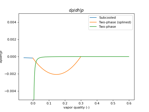
Two-Phase and Saturation Derivatives#
The two-phase derivatives of Thorade [188] are implemented in the CoolProp::AbstractState::first_two_phase_deriv() function, and derivatives along the saturation curve in the functions CoolProp::AbstractState::first_saturation_deriv() and CoolProp::AbstractState::second_saturation_deriv(). Here are some examples of using these functions:
In [35]: import CoolProp

In [36]: HEOS = CoolProp.AbstractState("HEOS", "Water")

In [37]: HEOS.update(CoolProp.QT_INPUTS, 0, 300)

# First saturation derivative calculated analytically
In [38]: HEOS.first_saturation_deriv(CoolProp.iP, CoolProp.iT)
Out[38]: 207.90345997878666

In [39]: HEOS.update(CoolProp.QT_INPUTS, 0, 300 + 0.001); p2 = HEOS.p()

In [40]: HEOS.update(CoolProp.QT_INPUTS, 0, 300 - 0.001); p1 = HEOS.p()

# First saturation derivative calculated numerically
In [41]: (p2-p1)/(2*0.001)
Out[41]: 207.90346005037463

In [42]: HEOS.update(CoolProp.QT_INPUTS, 0.1, 300)

# The d(Dmass)/d(Hmass)|P two-phase derivative
In [43]: HEOS.first_two_phase_deriv(CoolProp.iDmass, CoolProp.iHmass, CoolProp.iP)
Out[43]: -1.049411465836007e-06

# The d(Dmass)/d(Hmass)|P two-phase derivative using splines
In [44]: HEOS.first_two_phase_deriv_splined(CoolProp.iDmass, CoolProp.iHmass, CoolProp.iP, 0.3)
Out[44]: -0.0018169665165182374
An example of plotting these derivatives is here:
(Source code, png, .pdf)
Reference States#
To begin with, you should read the high-level docs about the reference state. Those docs are also applicable to the low-level interface.
Warning
As with the high-level interface, calling set_reference_stateS (or set_reference_state in python) should be called right at the beginning of your code, and not changed again later on.
Importantly, once an AbstractState-derived instance has been generated from the factory function, it DOES NOT pick up the change in the reference state. This is intentional, but you should watch out for this behavior.
Here is an example showing how to change the reference state and demonstrating the potential issues
In [45]: import CoolProp as CP

# This one doesn't see the change in reference state
In [46]: AS1 = CoolProp.AbstractState('HEOS','n-Propane');

In [47]: AS1.update(CoolProp.QT_INPUTS, 0, 233.15);

In [48]: CoolProp.CoolProp.set_reference_state('n-Propane','ASHRAE')

# This one gets the update in the reference state
In [49]: AS2 = CoolProp.AbstractState('HEOS','n-Propane');

In [50]: AS2.update(CoolProp.QT_INPUTS, 0, 233.15);

# Note how the AS1 has its default value (change in reference state is not seen)
# and AS2 does see the new reference state
In [51]: print('{0}, {1}'.format(AS1.hmass(), AS2.hmass()))
105123.2721376161, -1.464219296919336e-11

# Back to the original value
In [52]: CoolProp.CoolProp.set_reference_state('n-Propane','DEF')
Low-level interface using REFPROP#
If you have the REFPROP library installed, you can call REFPROP in the same way that you call CoolProp, but with REFPROP as the backend instead of HEOS. For instance, as in python:
In [53]: import CoolProp

In [54]: REFPROP = CoolProp.AbstractState("REFPROP", "WATER")

In [55]: REFPROP.update(CoolProp.DmolarT_INPUTS, 1e-6, 300)

In [56]: REFPROP.p(), REFPROP.hmass(), REFPROP.hmolar()
Out[56]: (0.0024943114042796856, 2551431.068564326, 45964.71448371271)

In [57]: [REFPROP.keyed_output(k) for k in [CoolProp.iP, CoolProp.iHmass, CoolProp.iHmolar]]
Out[57]: [0.0024943114042796856, 2551431.068564326, 45964.71448371271]
Access from High-Level Interface#
For languages that cannot directly instantiate C++ classes or their wrappers but can call a DLL (Excel, FORTRAN, Julia, etc. ) an interface layer has been developed. These functions can be found in CoolPropLib.h, and all these function names start with AbstractState. A somewhat limited subset of the functionality has been implemented, if more functionality is desired, please open an issue at CoolProp/CoolProp#issues. Essentially, this interface generates AbstractState pointers that are managed internally, and the interface allows you to call the methods of the low-level instances.
Here is an example of the shared library usage with Julia wrapper:
julia> import CoolProp

julia> PT_INPUTS = CoolProp.get_input_pair_index("PT_INPUTS")
7

julia> cpmass = CoolProp.get_param_index("C")
34

julia> handle = CoolProp.AbstractState_factory("HEOS", "Water")
0

julia> CoolProp.AbstractState_update(handle,PT_INPUTS,101325, 300)

julia> CoolProp.AbstractState_keyed_output(handle,cpmass)
4180.635776569655

julia> CoolProp.AbstractState_free(handle)

julia> handle = CoolProp.AbstractState_factory("HEOS", "Water&Ethanol")
1

julia> PQ_INPUTS = CoolProp.get_input_pair_index("PQ_INPUTS")
2

julia> T = CoolProp.get_param_index("T")
18

julia> CoolProp.AbstractState_set_fractions(handle, [0.4, 0.6])

julia> CoolProp.AbstractState_update(handle,PQ_INPUTS,101325, 0)

julia> CoolProp.AbstractState_keyed_output(handle,T)
352.3522142890429

julia> CoolProp.AbstractState_free(handle)
The call to AbstractState_free is not strictly needed as all managed AbstractState instances will auto-deallocate. But if you are generating thousands or millions of AbstractState instances in this fashion, you might want to tidy up periodically.
Here is a further example in C++:
#include "CoolPropLib.h"
#include "CoolPropTools.h"
#include <vector>
#include <time.h>

int main() {
    double t1, t2;
    const long buffersize = 500;
    long errcode = 0;
    char buffer[buffersize];
    long handle = AbstractState_factory("BICUBIC&HEOS", "Water", &errcode, buffer, buffersize);
    long _HmassP = get_input_pair_index("HmassP_INPUTS");
    long _Dmass = get_param_index("Dmass");
    long len = 20000;
    std::vector<double> h = linspace(700000.0, 1500000.0, len);
    std::vector<double> p = linspace(2.8e6, 3.0e6, len);
    double summer = 0;
    t1 = clock();
    for (long i = 0; i < len; ++i) {
        AbstractState_update(handle, _HmassP, h[i], p[i], &errcode, buffer, buffersize);
        summer += AbstractState_keyed_output(handle, _Dmass, &errcode, buffer, buffersize);
    }
    t2 = clock();
    std::cout << format("value(all): %0.13g, %g us/call\n", summer, ((double)(t2 - t1)) / CLOCKS_PER_SEC / double(len) * 1e6);
    return EXIT_SUCCESS;
}
which yields the output:
value(all): 8339004.432514, 0.8 us/call
Here is a further example in C++ that shows how to obtain many output variables at the same time, either 5 common outputs, or up to 5 user-selected vectors:
#include "CoolPropLib.h"
#include "CoolPropTools.h"
#include <vector>
#include <time.h>

int main() {
    const long buffer_size = 1000, length = 100000;
    long ierr;
    char herr[buffer_size];
    long handle = AbstractState_factory("BICUBIC&HEOS", "Water", &ierr, herr, buffer_size);
    std::vector<double> T(length), p(length), rhomolar(length), hmolar(length), smolar(length);
    std::vector<double> input1 = linspace(700000.0, 1500000.0, length);
    std::vector<double> input2 = linspace(2.8e6, 3.0e6, length);
    long input_pair = get_input_pair_index("HmassP_INPUTS");
    double t1 = clock();
    AbstractState_update_and_common_out(handle, input_pair, &(input1[0]), &(input2[0]), length, &(T[0]), &(p[0]), &(rhomolar[0]), &(hmolar[0]),
                                        &(smolar[0]), &ierr, herr, buffer_size);
    double t2 = clock();
    std::cout << format("value(commons): %g us/call\n", ((double)(t2 - t1)) / CLOCKS_PER_SEC / double(length) * 1e6);

    std::vector<long> outputs(5);
    outputs[0] = get_param_index("T");
    outputs[1] = get_param_index("P");
    outputs[2] = get_param_index("Dmolar");
    outputs[3] = get_param_index("Hmolar");
    outputs[4] = get_param_index("Smolar");
    std::vector<double> out1(length), out2(length), out3(length), out4(length), out5(length);
    t1 = clock();
    AbstractState_update_and_5_out(handle, input_pair, &(input1[0]), &(input2[0]), length, &(outputs[0]), &(out1[0]), &(out2[0]), &(out3[0]),
                                   &(out4[0]), &(out5[0]), &ierr, herr, buffer_size);
    t2 = clock();
    std::cout << format("value(user-specified): %g us/call\n", ((double)(t2 - t1)) / CLOCKS_PER_SEC / double(length) * 1e6);
}
which yields the output:
value(commons): 0.78 us/call
value(user-specified): 0.78 us/call