Tabular Interpolation¶

Especially when evaluating inputs as a function of pressure and enthalpy (common in many engineering applications), evaluation of the full equation of state is simply too slow, and it is necessary to come up with some means to speed up the calculations.

As of version 5.1 of CoolProp, the tabular interpolation methods of CoolProp v4 have been brought back from the dead, and significantly improved. They are approximately 4 times faster than the equivalent methods in v4 of CoolProp due to a more optimized structure. In order to make the most effective use of the tabular interpolation methods, you must be using the low-level interface, otherwise significant overhead and slowdown will be experienced. Thus, this method is best suited to C++, python, and the SWIG wrappers.

There are two backends implemented for tabular interpolation, BICUBIC and TTSE. Both consume the same gridded tabular data that is stored to your user home directory in the folder HOME/.CoolProp/Tables. If you want to find the directory that CoolProp is using as your home directory (HOME), you can do something like

In [1]: import CoolProp.CoolProp as CP

In [2]: CP.get_global_param_string("HOME")
Out[2]: '/github/home'

This directory is used because the user should under almost all circumstances have read/write access to this folder. Alternatively, if for some reason you want to use a different directory, you can set the configuration variable ALTERNATIVE_TABLES_DIRECTORY (see Configuration Variables).

Warning

Constructing the tables generates approximately 20 MB of data per fluid. The size of the directory of tabular data can get to be quite large if you use tables with lots of fluids. By default, CoolProp will warn when this directory is greater than 1 GB in size, and error out at 1.5 x (1.0 GB). This cap can be lifted by setting a configuration variable (see Configuration Variables) as shown here

In [3]: import CoolProp.CoolProp as CP, json

In [4]: jj = json.loads(CP.get_config_as_json_string())

In [5]: jj['MAXIMUM_TABLE_DIRECTORY_SIZE_IN_GB'] = 1.0

In [6]: jj = CP.set_config_as_json_string(json.dumps(jj))

General Information¶

Two sets of tables are generated and written to disk: pressure-enthalpy and pressure-temperature tables. The tables are generated over the full range of temperatures between the triple point temperature and the maximum temperature, with pressures from the minimum pressure to the maximum pressure. Pressure-enthalpy and pressure-temperature will be the fastest inputs with these methods because they are the so-called native inputs of the tables. Other inputs, such as pressure-entropy, require an additional iteration, though the overhead is not as severe as for the full equation of state.

It is critical that you try to only initialize one AbstractState instance and then call its methods. The overhead for generating an AbstractState instance when using TTSE or BICUBIC is not too punitive, but you should try to only do it once. Each time an instance is generated, all the tabular data is loaded into it.

TTSE Interpolation¶

The basic concept behind Tabular Taylor Series Extrapolation (TTSE) extrapolation is that you cache the value and its derivatives with respect to a set of two variables over a regularly (linearly or logarithmically) spaced grid. It is therefore easy to look up the index of the independent variables x and y by interval bisection. Once the coordinates of the given grid point \(i,j\) are known, you can used the cached derivatives of the desired variable \(z\) to obtain it in terms of the given independent variables \(x\) and \(y\):

\[z = z_{i,j}+\Delta x\left(\frac{\partial z}{\partial x}\right)_{y}+\Delta y\left(\frac{\partial z}{\partial y}\right)_{x}+\frac{1}{2}\Delta x^2\left(\frac{\partial^2 z}{\partial x^2}\right)_{y}+\frac{1}{2}\Delta y^2\left(\frac{\partial^2z}{\partial y^2}\right)_{y}+\Delta x\Delta y\left(\frac{\partial^2z}{\partial y\partial x}\right)\]

\[ \begin{align}\begin{aligned}\Delta x = x-x_i\\\Delta x = y-y_j\end{aligned}\end{align} \]

See the IAPWS TTSE report for a description of the method. Analytic derivatives are used to build the tables

Bicubic Interpolation¶

In bicubic interpolation, the values of the output parameter as well as its derivatives are evaluated at the corners of a unit square, and these values are used to fit a bicubic surface over the unit square. Wikipedia has excellent coverage of bicubic interpolation, and the method implemented in CoolProp is exactly this method.

Normalized cell values are generated from

\[ \begin{align}\begin{aligned}\hat x = \frac{x-x_i}{x_{i+1}-x_{i}}\\\hat y = \frac{y-y_j}{y_{j+1}-y_{j}}\end{aligned}\end{align} \]

And derivatives must be scaled to be in terms of unit cell values, or

\[ \begin{align}\begin{aligned}\frac{\partial z}{\partial \hat x} = \frac{\partial z}{\partial x}\frac{\partial x}{\partial \hat x}\\\frac{\partial z}{\partial \hat y} = \frac{\partial z}{\partial y}\frac{\partial y}{\partial \hat y}\end{aligned}\end{align} \]

In CoolProp, after loading the tabular data, the coefficients for all cells are calculated in one shot.

Accuracy comparison¶

Here is a simple comparison of accuracy, the density is obtained for R245fa using the EOS, TTSE extrapolation, and Bicubic interpolation

In [7]: import CoolProp

In [8]: HEOS = CoolProp.AbstractState("HEOS", "R245fa")

In [9]: TTSE = CoolProp.AbstractState("TTSE&HEOS", "R245fa")

In [10]: BICU = CoolProp.AbstractState("BICUBIC&HEOS", "R245fa")

In [11]: HEOS.update(CoolProp.PT_INPUTS, 101325, 300); BICU.update(CoolProp.PT_INPUTS, 101325, 300); TTSE.update(CoolProp.PT_INPUTS, 101325, 300)

In [12]: print(HEOS.rhomolar(), TTSE.rhomolar(), BICU.rhomolar())
42.13513665749303 42.13502246599472 42.13513655671527

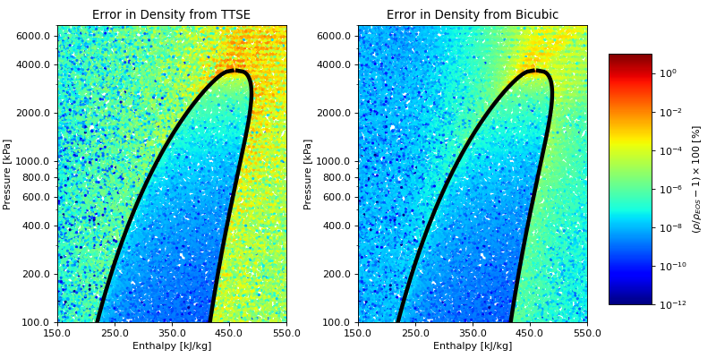
A more complete comparison of the accuracy of these methods can be obtained by studying the following figure for refrigerant R245fa. You can download the script and change the fluid name to another fluid to investigate the behavior

(Source code, png, .pdf)

Speed comparison¶

The primary motivation for the use of tabular interpolation is the improvement in computational speed. Thus a small summary could be useful. This tabular data was obtained by this python script : (link to script).

R245fa : 50000 calls, best of 3 repetitions

Execution speed in \(\mu\) s/call¶
Backend	2-Phase p-h inputs	1-phase p-h inputs	1-phase p-T inputs
`HEOS`	63.51	23.48	4.07
`TTSE&HEOS`	0.33	0.35	0.38
`BICUBIC&HEOS`	0.33	0.34	0.38

More Information¶

The tables are stored in a zipped format using the msgpack package and miniz. If you want to see what data is serialized in the tabular data, you can unzip and unpack into python (or other high-level languages) using something roughly like:

import msgpack, zlib, io, numpy as np, matplotlib.pyplot as plt

root = r'C:\Users\ian\.CoolProp\Tables\REFPROPMixtureBackend(R32[0.8292500000]&R1234yf[0.1707500000])'
with open(root+'/single_phase_logph.bin.z','rb') as fp:
    values = msgpack.load(io.BytesIO(zlib.decompress(fp.read())))
    revision, matrices = values[0:2]
    T,h,p,rho = np.array(matrices['T']), np.array(matrices['hmolar']), np.array(matrices['p']), np.array(matrices['rhomolar'])
    plt.plot(np.array(matrices['p']),np.array(matrices['hmolar']),'x')
with open(root+'/phase_envelope.bin.z','rb') as fp:
    values = msgpack.load(io.BytesIO(zlib.decompress(fp.read())))
    revision, matrices = values[0:2]
    plt.plot(np.array(matrices['p']),np.array(matrices['hmolar_vap']),'-')
plt.show()

with open(root+'/single_phase_logpT.bin.z','rb') as fp:
    values = msgpack.load(io.BytesIO(zlib.decompress(fp.read())))
    revision, matrices = values[0:2]
    T,h,p,rho = np.array(matrices['T']), np.array(matrices['hmolar']), np.array(matrices['p']), np.array(matrices['rhomolar'])
    plt.plot(np.array(matrices['p']),np.array(matrices['T']),'x')
with open(root+'/phase_envelope.bin.z','rb') as fp:
    values = msgpack.load(io.BytesIO(zlib.decompress(fp.read())))
    revision, matrices = values[0:2]
    plt.plot(np.array(matrices['p']),np.array(matrices['T']),'-')
plt.show()

You’ll need msgpack wrapper for your target language.