High-Level Interface ¶

PropsSI function ¶

For many users, all that is needed is a simple call to the PropsSI function for pure fluids, pseudo-pure fluids and mixtures. For humid air properties, see Humid air properties. An example using PropsSI:

# Import the PropsSI function
In [1]: from CoolProp.CoolProp import PropsSI

# Saturation temperature of Water at 1 atm in K
In [2]: PropsSI('T','P',101325,'Q',0,'Water')
Out[2]: 373.1242958476844

In this example, the first parameter, \(T\), is the output property that will be returned from PropsSI. The second and fourth parameters are the specified input pair of properties that determine the state point where the output property will be calculated. The output property and input pair properties are text strings and must be quoted. The third and fifth parameters are the values of the input pair properties and will determine the state point. The sixth and last parameter is the fluid for which the output property will be calculated; also a quoted string.

More information:

All the wrappers wrap this function in exactly the same way.

For pure and pseudo-pure fluids, two state variables are required to fix the state. The equations of state are based on \(T\) and \(\rho\) as state variables, so \(T, \rho\) will always be the fastest inputs. \(P,T\) will be a bit slower (3-10 times), followed by input pairs where neither \(T\) nor \(\rho\) are specified, like \(P,H\); these will be much slower. If speed is an issue, you can look into table-based interpolation methods using TTSE or bicubic interpolation; or if you are only interested in Water properties, you can look into using the IF97 (industrial formulation) backend.

Vapor, Liquid, and Saturation States ¶

If the input pair (say, \(P,T\)) defines a state point that lies in the vapor region, then the vapor property at that state point will be returned. Likewise, if the state point lies in the liquid region, then the liquid state property at that state point will be returned. If the state point defined by the input pair lies within 1E-4 % of the saturation pressure, then CoolProp may return an error, because both liquid and vapor are defined along the saturation curve.

To retrieve either the vapor or liquid properties along the saturation curve, provide an input pair that includes either the saturation temperature, \(T\), or saturation pressure, \(p\), along with the vapor quality, \(Q\). Use a value of \(Q=1\) for the saturated vapor property or \(Q=0\) for the saturated liquid property. For example, at a saturation pressure of 1 atm, the liquid and vapor enthalpies can be returned as follows.

# Import the PropsSI function
In [3]: from CoolProp.CoolProp import PropsSI

# Saturated vapor enthalpy of Water at 1 atm in J/kg
In [4]: H_V = PropsSI('H','P',101325,'Q',1,'Water'); print(H_V)
2675529.3255007486

# Saturated liquid enthalpy of Water at 1 atm in J/kg
In [5]: H_L = PropsSI('H','P',101325,'Q',0,'Water'); print(H_L)
419057.7330940691

# Latent heat of vaporization of Water at 1 atm in J/kg
In [6]: H_V - H_L
Out[6]: 2256471.5924066794

Note

The latent heat of vaporization can be calculated using the difference between the vapor and liquid enthalpies at the same point on the saturation curve.

Imposing the Phase (Optional)¶

Each call to PropsSI() requires the phase to be determined based on the provided input pair, and may require a non-trivial flash calculation to determine if the state point is in the single-phase or two-phase region and to generate a sensible initial guess for the solver. For computational efficiency, PropsSI() allows the phase to be manually imposed through the input key parameters. If unspecified, PropsSI will attempt to determine the phase automatically.

Depending on the input pair, there may or may not be a speed benefit to imposing a phase. However, some state points may not be able to find a suitable initial guess for the solver and being able to impose the phase manually may offer a solution if the solver is failing. Additionally, with an input pair in the two-phase region, it can be useful to impose a liquid or gas phase to instruct PropsSI() to return the saturated liquid or saturated gas properties.

To specify the phase to be used, add the “|” delimiter to one (and only one) of the input key strings followed by one of the phase strings in the table below:

Phase String	Phase Region
“liquid”	p < pcrit & T < Tcrit ; above saturation
“gas”	p < pcrit & T < Tcrit ; below saturation
“twophase”	p < pcrit & T < Tcrit ; mixed liquid/gas
“supercritical_liquid”	p > pcrit & T < Tcrit
“supercritical_gas”	p < pcrit & T > Tcrit
“supercritical”	p > pcrit & T > Tcrit
“not_imposed”	(Default) CoolProp to determine phase

For example:

# Get the density of Water at T = 461.1 K and P = 5.0e6 Pa, imposing the liquid phase
In [7]: PropsSI('D','T|liquid',461.1,'P',5e6,'Water')
Out[7]: 881.000853334732

# Get the density of Water at T = 597.9 K and P = 5.0e6 Pa, imposing the gas phase
In [8]: PropsSI('D','T',597.9,'P|gas',5e6,'Water')
Out[8]: 20.508496070580005

On each call to PropsSI(), the imposed phase is reset to “not_imposed” as long as no imposed phase strings are used. A phase string must be appended to an Input key string on each and every call to PropsSI() to impose the phase. PropsSI() will return an error for any of the following syntax conditions:

If anything other than the pipe, “|”, symbol is used as the delimiter
If the phase string is not one of the valid phase strings in the table above
If the phase string is applied to more than one of the Input key parameters

In addition, for consistency with the low-level interface, the valid phase strings in the table above may be prefixed with either “phase_” or “iphase_” and still be recognized as a valid phase string.

Warning

When specifying an imposed phase, it is absolutely critical that the input pair actually lie within the imposed phase region. If an incorrect phase is imposed for the given input pair, PropsSI() may throw unexpected errors or incorrect results may possibly be returned from the property functions. If the state point phase is not absolutely known, it is best to let CoolProp determine the phase.

Fluid information ¶

You can obtain string-encoded information about the fluid from the get_fluid_param_string function with something like:

In [9]: import CoolProp.CoolProp as CP

In [10]: for k in ['formula','CAS','aliases','ASHRAE34','REFPROP_name','pure','INCHI','INCHI_Key','CHEMSPIDER_ID']:
   ....:     item = k + ' --> ' + CP.get_fluid_param_string("R125", k)
   ....:     print(item)
   ....: 
formula --> C_{2}F_{5}H_{1}
CAS --> 354-33-6
aliases --> 
ASHRAE34 --> UNKNOWN
REFPROP_name --> R125
pure --> true
INCHI --> InChI=1S/C2HF5/c3-1(4)2(5,6)7/h1H
INCHI_Key --> GTLACDSXYULKMZ-UHFFFAOYSA-N
CHEMSPIDER_ID --> 9256

Trivial inputs ¶

In order to obtain trivial inputs that do not depend on the thermodynamic state, in wrappers that support the Props1SI function, you can obtain the trivial parameter (in this case the critical temperature of water) like:

Props1SI(“Tcrit”,”Water”)

In python, the PropsSI function is overloaded to also accept two inputs:

In [11]: import CoolProp.CoolProp as CP

In [12]: CP.PropsSI("Tcrit","Water")
Out[12]: 647.096

In [13]: CP.PropsSI("Tcrit","REFPROP::WATER")
Out[13]: 647.096

Furthermore, you can in all languages call the PropsSI function directly using dummy arguments for the other unused parameters:

In [14]: import CoolProp.CoolProp as CP

In [15]: CP.PropsSI("Tcrit","",0,"",0,"Water")
Out[15]: 647.096

PhaseSI function ¶

It can be useful to know what the phase of a given state point is. A high-level function called PhaseSI has been implemented to allow for access to the phase.

In [16]: import CoolProp.CoolProp as CP

In [17]: CP.PhaseSI('P',101325,'Q',0,'Water')
Out[17]: 'twophase'

The phase index (as floating point number) can also be obtained using the PropsSI function. In python you would do:

In [18]: import CoolProp.CoolProp as CP

In [19]: CP.PropsSI('Phase','P',101325,'Q',0,'Water')
Out[19]: 6.0

where you can obtain the integer indices corresponding to the phase flags using the get_phase_index function:

In [20]: import CoolProp.CoolProp as CP

In [21]: CP.get_phase_index('phase_twophase')
Out[21]: 6

# Or for liquid
In [22]: CP.get_phase_index('phase_liquid')
Out[22]: 0

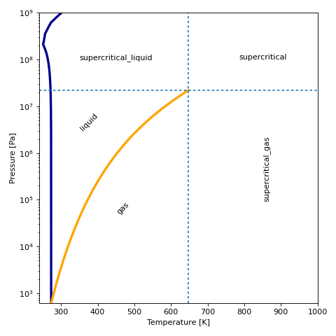
For a given fluid, the phase can be plotted in T-p coordinates:

(Source code, png, .pdf)

Partial Derivatives ¶

First Partial Derivatives for Single-phase States¶

For some applications it can be useful to have access to partial derivatives of thermodynamic properties. A generalized first partial derivative has been implemented into CoolProp, which can be obtained using the PropsSI function by encoding the desired derivative as a string. The format of the string is d(OF)/d(WRT)|CONSTANT which is the same as

\[\left. \frac{\partial OF}{\partial WRT}\right|_{CONSTANT}\]

At the low-level, the CoolProp code calls the function AbstractState::first_partial_deriv(). Refer to the function documentation to see how the generalized derivative works.

Warning

This derivative formulation is currently only valid for homogeneous (single-phase) states. Two phase derivatives are not defined, and are for many combinations, invalid.

Here is an example of calculating the constant pressure specific heat, which is defined by the relation

\[c_p = \left.\frac{\partial h}{\partial T}\right|_{p}\]

and called through python

In [23]: import CoolProp.CoolProp as CP

# c_p using c_p
In [24]: CP.PropsSI('C','P',101325,'T',300,'Water')
Out[24]: 4180.6357765560715

# c_p using derivative
In [25]: CP.PropsSI('d(Hmass)/d(T)|P','P',101325,'T',300,'Water')
Out[25]: 4180.6357765560715

It is also possible to call the derivatives directly using the low-level partial derivatives functionality. The low-level routine is in general faster because it avoids the string parsing.

Second Partial Derivatives for Single-Phase States¶

In a similar fashion it is possible to evaluate second derivatives. For instance, the derivative of \(c_p\) with respect to mass-based specific enthalpy at constant pressure could be obtained by

In [26]: import CoolProp.CoolProp as CP

# c_p using derivative
In [27]: CP.PropsSI('d(d(Hmass)/d(T)|P)/d(Hmass)|P','P',101325,'T',300,'Water')
Out[27]: -7.767989468924389e-05

where the inner part d(Hmass)/d(T)|P is the definition of \(c_p\).

Warning

This derivative formulation is currently only valid for homogeneous (single-phase) states. Two phase derivatives are not defined, and are for many combinations, invalid.

It is also possible to call the derivatives directly using the low-level partial derivatives functionality. The low-level routine is in general faster because it avoids the string parsing.

First Saturation Derivatives¶

It is also possible to retrieve the derivatives along the saturation curves using the high-level interface, encoding the desired derivative as a string just like for the single-phase derivatives.

Warning

This derivative formulation is currently only valid for saturated states where the vapor quality is either 0 or 1.

For instance, to calculate the saturation derivative of enthalpy ALONG the saturated vapor curve, you could do:

In [28]: import CoolProp

In [29]: CoolProp.CoolProp.PropsSI('d(Hmolar)/d(T)|sigma','P',101325,'Q',1,'Water')
Out[29]: 28.427795995713694

It is also possible to call the derivatives directly using the low-level partial derivatives functionality. The low-level routine is in general faster because it avoids the string parsing.

Predefined Mixtures ¶

A number of predefined mixtures are included in CoolProp. You can retrieve the list of predefined mixtures by calling get_global_param_string("predefined_mixtures") which will return a comma-separated list of predefined mixtures. In Python, to get the first 6 mixtures, you would do

In [30]: import CoolProp.CoolProp as CP

In [31]: CP.get_global_param_string('predefined_mixtures').split(',')[0:6]
Out[31]: 
['AIR.MIX',
 'AMARILLO.MIX',
 'Air.mix',
 'Amarillo.mix',
 'EKOFISK.MIX',
 'Ekofisk.mix']

and then to calculate the density of air using the mixture model at 1 atmosphere (=101325 Pa) and 300 K, you could do

In [32]: import CoolProp.CoolProp as CP

In [33]: CP.PropsSI('D','P',101325,'T',300,'Air.mix')
Out[33]: 1.1766922904316655

Exactly the same methodology can be used from other wrappers.

User-Defined Mixtures ¶

When using mixtures in CoolProp, you can specify mixture components and composition by encoding the mixture components and mole fractions by doing something like

In [34]: import CoolProp.CoolProp as CP

In [35]: CP.PropsSI('D','T',300,'P',101325,'HEOS::R32[0.697615]&R125[0.302385]')
Out[35]: 2.986886779635724

You can handle ternary and multi-component mixtures in the same fashion, just add the other components to the fluid string with a & separating components and the fraction of the component in [ and ] brackets

Reference States ¶

Enthalpy and entropy are relative properties! You should always be comparing differences in enthalpy rather than absolute values of the enthalpy or entropy. That said, if can be useful to set the reference state values for enthalpy and entropy to one of a few standard values. This is done by the use of the set_reference_state function in python, or the set_reference_stateS function most everywhere else. For documentation of the underlying C++ function, see CoolProp::set_reference_stateS().

Warning

The changing of the reference state should be part of the initialization of your program, and it is not recommended to change the reference state during the course of making calculations

A number of reference states can be used:

IIR: h = 200 kJ/kg, s=1 kJ/kg/K at 0C saturated liquid
ASHRAE: h = 0, s = 0 @ -40C saturated liquid
NBP: h=0, s=0 for saturated liquid at 1 atmosphere
DEF: Go back to the default reference state for the fluid

which can be used like

In [36]: import CoolProp.CoolProp as CP

In [37]: CP.set_reference_state('n-Propane','ASHRAE')

# Should be zero (or very close to it)
In [38]: CP.PropsSI('H', 'T', 233.15, 'Q', 0, 'n-Propane')
Out[38]: 2.928438593838672e-11

# Back to the original value
In [39]: CP.set_reference_state('n-Propane','DEF')

# Should not be zero
In [40]: CP.PropsSI('H', 'T', 233.15, 'Q', 0, 'n-Propane')
Out[40]: 105123.27213761522

For non-standard reference states, you can specify them directly for the given temperature and molar(!) density. Here is an example of setting the enthalpy and entropy at 298.15 K and 1 atm to some specified values

In [41]: import CoolProp.CoolProp as CP

In [42]: Dmolar = CP.PropsSI("Dmolar", "T", 298.15, "P", 101325, "NH3")

In [43]: CP.set_reference_state('NH3', 298.15, Dmolar, -60000.12, 314.159) # fluid, T, D (mol/m^3), h (J/mol), s (J/mol/K)

In [44]: CP.PropsSI("Hmolar", "T", 298.15, "P", 101325, "NH3")
Out[44]: -60000.119999999995

In [45]: CP.PropsSI("Smolar", "T", 298.15, "P", 101325, "NH3")
Out[45]: 314.15900000000005

# Back to the original value
In [46]: CP.set_reference_state('NH3','DEF')

Calling REFPROP ¶

If you have the REFPROP library installed, you can call REFPROP in the same way that you call CoolProp, but with REFPROP:: preceding the fluid name. For instance, as in python:

In [47]: import CoolProp.CoolProp as CP

# Using properties from CoolProp to get R410A density
In [48]: CP.PropsSI('D','T',300,'P',101325,'HEOS::R32[0.697615]&R125[0.302385]')
Out[48]: 2.986886779635724

# Using properties from REFPROP to get R410A density
In [49]: CP.PropsSI('D','T',300,'P',101325,'REFPROP::R32[0.697615]&R125[0.302385]')
Out[49]: 2.9868867801892165

Adding Fluids ¶

The fluids in CoolProp are all compiled into the library itself, and are given in the JSON format. They are all stored in the dev/fluids folder relative to the root of the repository. If you want to obtain the JSON data for a fluid from CoolProp, print out a part of it, and then load it back into CoolProp, you could do:

In [50]: import CoolProp.CoolProp as CP

# Get the JSON structure for Water
In [51]: jj = CP.get_fluid_param_string("Water", "JSON")

# Now load it back into CoolProp - Oops! This isn't going to work because it is already there.
In [52]: CP.add_fluids_as_JSON("HEOS", jj)
---------------------------------------------------------------------------
RuntimeError                              Traceback (most recent call last)
Cell In [52], line 1
----> 1 CP.add_fluids_as_JSON("HEOS", jj)

File CoolProp/CoolProp.pyx:303, in CoolProp.CoolProp.add_fluids_as_JSON()

File CoolProp/CoolProp.pyx:307, in CoolProp.CoolProp.add_fluids_as_JSON()

RuntimeError: Unable to load fluid [Water] due to error: Cannot load fluid [Water:7732-18-5] because it is already in library; index = [15] of [124]; Consider enabling the config boolean variable OVERWRITE_FLUIDS

# Set the configuration variable allowing for overwriting
In [53]: CP.set_config_bool(CP.OVERWRITE_FLUIDS, True)

# Now load it back into CoolProp - Success!
In [54]: CP.add_fluids_as_JSON("HEOS", jj)

# Turn overwriting back off
In [55]: CP.set_config_bool(CP.OVERWRITE_FLUIDS, False)

C++ Sample Code ¶

#include "CoolProp.h"
#include <iostream>
#include <stdlib.h>
using namespace CoolProp;
int main() {
    // First type (slowest, due to most string processing, exposed in DLL)
    std::cout << PropsSI("Dmolar", "T", 298, "P", 1e5, "Propane[0.5]&Ethane[0.5]") << std::endl;  // Default backend is HEOS
    std::cout << PropsSI("Dmolar", "T", 298, "P", 1e5, "HEOS::Propane[0.5]&Ethane[0.5]") << std::endl;
    std::cout << PropsSI("Dmolar", "T", 298, "P", 1e5, "REFPROP::Propane[0.5]&Ethane[0.5]") << std::endl;
    // Vector example
    std::vector<double> z(2, 0.5);
    // Second type (C++ only, a bit faster, allows for vector inputs and outputs)
    std::vector<std::string> fluids;
    fluids.push_back("Propane");
    fluids.push_back("Ethane");
    std::vector<std::string> outputs;
    outputs.push_back("Dmolar");
    std::vector<double> T(1, 298), p(1, 1e5);
    std::cout << PropsSImulti(outputs, "T", T, "P", p, "", fluids, z)[0][0] << std::endl;  // Default backend is HEOS
    std::cout << PropsSImulti(outputs, "T", T, "P", p, "HEOS", fluids, z)[0][0] << std::endl;
    // Comment me out if REFPROP is not installed
    std::cout << PropsSImulti(outputs, "T", T, "P", p, "REFPROP", fluids, z)[0][0] << std::endl;
    // All done return
    return EXIT_SUCCESS;
}

C++ Sample Code Output ¶

Sample Code ¶

In [56]: import CoolProp as CP

In [57]: print(CP.__version__)
6.6.1dev

In [58]: print(CP.__gitrevision__)
956d949bbdd4c2b6093f67bd02ece896c9c35b0a

#Import the things you need
In [59]: from CoolProp.CoolProp import PropsSI

# Specific heat (J/kg/K) of 20% ethylene glycol as a function of T
In [60]: PropsSI('C','T',298.15,'P',101325,'INCOMP::MEG-20%')
Out[60]: 3905.2706242925874

# Density of Air at standard atmosphere in kg/m^3
In [61]: PropsSI('D','T',298.15,'P',101325,'Air')
Out[61]: 1.1843184839089664

# Saturation temperature of Water at 1 atm
In [62]: PropsSI('T','P',101325,'Q',0,'Water')
Out[62]: 373.1242958476844

# Saturated vapor enthalpy of R134a at 0C (Q=1)
In [63]: PropsSI('H','T',273.15,'Q',1,'R134a')
Out[63]: 398603.45362765493

# Saturated liquid enthalpy of R134a at 0C (Q=0)
In [64]: PropsSI('H','T',273.15,'Q',0,'R134a')
Out[64]: 199999.98852614488

# Using properties from CoolProp to get R410A density
In [65]: PropsSI('D','T',300,'P',101325,'HEOS::R32[0.697615]&R125[0.302385]')
Out[65]: 2.986886779635724

# Using properties from REFPROP to get R410A density
In [66]: PropsSI('D','T',300,'P',101325,'REFPROP::R32[0.697615]&R125[0.302385]')
Out[66]: 2.9868867801892165

# Check that the same as using pseudo-pure
In [67]: PropsSI('D','T',300,'P',101325,'R410A')
Out[67]: 2.986868076922677

# Using IF97 to get Water saturated vapor density at 100C
In [68]: PropsSI('D','T',400,'Q',1,'IF97::Water')
Out[68]: 1.3692496283046673

# Check the IF97 result using the default HEOS
In [69]: PropsSI('D','T',400,'Q',1,'Water')
Out[69]: 1.3694075410068227

Table of string inputs to PropsSI function ¶

Note

Please note that any parameter that is indicated as a trivial parameter can be obtained from the Props1SI function as shown above in Trivial inputs

Parameter	Units	Input/Output	Trivial	Description
`DELTA`, `Delta`		IO	False	Reduced density (rho/rhoc)
`DMOLAR`, `Dmolar`	mol/m^3	IO	False	Molar density
`D`, `DMASS`, `Dmass`	kg/m^3	IO	False	Mass density
`HMOLAR`, `Hmolar`	J/mol	IO	False	Molar specific enthalpy
`H`, `HMASS`, `Hmass`	J/kg	IO	False	Mass specific enthalpy
`P`	Pa	IO	False	Pressure
`Q`	mol/mol	IO	False	Molar vapor quality
`SMOLAR`, `Smolar`	J/mol/K	IO	False	Molar specific entropy
`S`, `SMASS`, `Smass`	J/kg/K	IO	False	Mass specific entropy
`TAU`, `Tau`		IO	False	Reciprocal reduced temperature (Tc/T)
`T`	K	IO	False	Temperature
`UMOLAR`, `Umolar`	J/mol	IO	False	Molar specific internal energy
`U`, `UMASS`, `Umass`	J/kg	IO	False	Mass specific internal energy
`ACENTRIC`, `acentric`		O	True	Acentric factor
`ALPHA0`, `alpha0`		O	False	Ideal Helmholtz energy
`ALPHAR`, `alphar`		O	False	Residual Helmholtz energy
`A`, `SPEED_OF_SOUND`, `speed_of_sound`	m/s	O	False	Speed of sound
`BVIRIAL`, `Bvirial`		O	False	Second virial coefficient
`CONDUCTIVITY`, `L`, `conductivity`	W/m/K	O	False	Thermal conductivity
`CP0MASS`, `Cp0mass`	J/kg/K	O	False	Ideal gas mass specific constant pressure specific heat
`CP0MOLAR`, `Cp0molar`	J/mol/K	O	False	Ideal gas molar specific constant pressure specific heat
`CPMOLAR`, `Cpmolar`	J/mol/K	O	False	Molar specific constant pressure specific heat
`CVIRIAL`, `Cvirial`		O	False	Third virial coefficient
`CVMASS`, `Cvmass`, `O`	J/kg/K	O	False	Mass specific constant volume specific heat
`CVMOLAR`, `Cvmolar`	J/mol/K	O	False	Molar specific constant volume specific heat
`C`, `CPMASS`, `Cpmass`	J/kg/K	O	False	Mass specific constant pressure specific heat
`D2ALPHA0_DDELTA2_CONSTTAU`, `d2alpha0_ddelta2_consttau`		O	False	Second derivative of ideal Helmholtz energy with delta
`D3ALPHA0_DDELTA3_CONSTTAU`, `d3alpha0_ddelta3_consttau`		O	False	Third derivative of ideal Helmholtz energy with delta
`DALPHA0_DDELTA_CONSTTAU`, `dalpha0_ddelta_consttau`		O	False	Derivative of ideal Helmholtz energy with delta
`DALPHA0_DTAU_CONSTDELTA`, `dalpha0_dtau_constdelta`		O	False	Derivative of ideal Helmholtz energy with tau
`DALPHAR_DDELTA_CONSTTAU`, `dalphar_ddelta_consttau`		O	False	Derivative of residual Helmholtz energy with delta
`DALPHAR_DTAU_CONSTDELTA`, `dalphar_dtau_constdelta`		O	False	Derivative of residual Helmholtz energy with tau
`DBVIRIAL_DT`, `dBvirial_dT`		O	False	Derivative of second virial coefficient with respect to T
`DCVIRIAL_DT`, `dCvirial_dT`		O	False	Derivative of third virial coefficient with respect to T
`DIPOLE_MOMENT`, `dipole_moment`	C m	O	True	Dipole moment
`FH`		O	True	Flammability hazard
`FRACTION_MAX`, `fraction_max`		O	True	Fraction (mole, mass, volume) maximum value for incompressible solutions
`FRACTION_MIN`, `fraction_min`		O	True	Fraction (mole, mass, volume) minimum value for incompressible solutions
`FUNDAMENTAL_DERIVATIVE_OF_GAS_DYNAMICS`, `fundamental_derivative_of_gas_dynamics`		O	False	Fundamental derivative of gas dynamics
`GAS_CONSTANT`, `gas_constant`	J/mol/K	O	True	Molar gas constant
`GMOLAR_RESIDUAL`, `Gmolar_residual`	J/mol/K	O	False	Residual molar Gibbs energy
`GMOLAR`, `Gmolar`	J/mol	O	False	Molar specific Gibbs energy
`GWP100`		O	True	100-year global warming potential
`GWP20`		O	True	20-year global warming potential
`GWP500`		O	True	500-year global warming potential
`G`, `GMASS`, `Gmass`	J/kg	O	False	Mass specific Gibbs energy
`HELMHOLTZMASS`, `Helmholtzmass`	J/kg	O	False	Mass specific Helmholtz energy
`HELMHOLTZMOLAR`, `Helmholtzmolar`	J/mol	O	False	Molar specific Helmholtz energy
`HH`		O	True	Health hazard
`HMOLAR_RESIDUAL`, `Hmolar_residual`	J/mol/K	O	False	Residual molar enthalpy
`ISENTROPIC_EXPANSION_COEFFICIENT`, `isentropic_expansion_coefficient`		O	False	Isentropic expansion coefficient
`ISOBARIC_EXPANSION_COEFFICIENT`, `isobaric_expansion_coefficient`	1/K	O	False	Isobaric expansion coefficient
`ISOTHERMAL_COMPRESSIBILITY`, `isothermal_compressibility`	1/Pa	O	False	Isothermal compressibility
`I`, `SURFACE_TENSION`, `surface_tension`	N/m	O	False	Surface tension
`M`, `MOLARMASS`, `MOLAR_MASS`, `MOLEMASS`, `molar_mass`, `molarmass`, `molemass`	kg/mol	O	True	Molar mass
`ODP`		O	True	Ozone depletion potential
`PCRIT`, `P_CRITICAL`, `Pcrit`, `p_critical`, `pcrit`	Pa	O	True	Pressure at the critical point
`PHASE`, `Phase`		O	False	Phase index as a float
`PH`		O	True	Physical hazard
`PIP`		O	False	Phase identification parameter
`PMAX`, `P_MAX`, `P_max`, `pmax`	Pa	O	True	Maximum pressure limit
`PMIN`, `P_MIN`, `P_min`, `pmin`	Pa	O	True	Minimum pressure limit
`PRANDTL`, `Prandtl`		O	False	Prandtl number
`PTRIPLE`, `P_TRIPLE`, `p_triple`, `ptriple`	Pa	O	True	Pressure at the triple point (pure only)
`P_REDUCING`, `p_reducing`	Pa	O	True	Pressure at the reducing point
`RHOCRIT`, `RHOMASS_CRITICAL`, `rhocrit`, `rhomass_critical`	kg/m^3	O	True	Mass density at critical point
`RHOMASS_REDUCING`, `rhomass_reducing`	kg/m^3	O	True	Mass density at reducing point
`RHOMOLAR_CRITICAL`, `rhomolar_critical`	mol/m^3	O	True	Molar density at critical point
`RHOMOLAR_REDUCING`, `rhomolar_reducing`	mol/m^3	O	True	Molar density at reducing point
`SMOLAR_RESIDUAL`, `Smolar_residual`	J/mol/K	O	False	Residual molar entropy (sr/R = s(T,rho) - s^0(T,rho))
`TCRIT`, `T_CRITICAL`, `T_critical`, `Tcrit`	K	O	True	Temperature at the critical point
`TMAX`, `T_MAX`, `T_max`, `Tmax`	K	O	True	Maximum temperature limit
`TMIN`, `T_MIN`, `T_min`, `Tmin`	K	O	True	Minimum temperature limit
`TTRIPLE`, `T_TRIPLE`, `T_triple`, `Ttriple`	K	O	True	Temperature at the triple point
`T_FREEZE`, `T_freeze`	K	O	True	Freezing temperature for incompressible solutions
`T_REDUCING`, `T_reducing`	K	O	True	Temperature at the reducing point
`V`, `VISCOSITY`, `viscosity`	Pa s	O	False	Viscosity
`Z`		O	False	Compressibility factor